A while back I was debugging some legacy code. Profiling revealed that a few lines of code that computes “connected components” was a major bottleneck.

Here, the concept of “connected components” is simple: suppose we have a number of sets, some of which overlap; we’ll union any two sets that overlap, and do this recursively; in the end, we’ll get a number of non-ovrlapping sets, and they are called “connected components”.

To fix the terminology, we’ll call the original sets components, the final non-overalapping sets (i.e. “connected components”) groups, and elements in the sets items.

The code uses a python package called networkx; it’s as simple as the following:

1
2
3
4
5
6
7
8
9
10
11
12
# module cc_nx

from typing import Iterable
import networkx as nx


def connected_components(components: Iterable[Iterable[int]]):
    graph = nx.parse_adjlist(
            (' '.join(str(i) for i in c) for c in components),
            nodetype=int,
            )
    return list(nx.connected_components(graph))

Let’s see it in action:

1
2
3
4
5
6
7
8
9
10
11
12
13
>>> COMPONENTS = [
...     (0, 1, 2, 3, 4, 5),
...     (0, 1, 8),
...     (2, 9),
...     (6, 7),
...     (5,),
...     (8, 9),
...     (10, 11, 12, 13),
...     (10, 14, 15),
...     ]
>>> from cc_nx import connected_components
>>> connected_components(COMPONENTS)
[{0, 1, 2, 3, 4, 5, 8, 9}, {6, 7}, {10, 11, 12, 13, 14, 15}]

To make it a little more interesting and realistic, let’s randomize the order of the elements:

1
2
3
4
5
6
7
8
9
10
11
12
>>> COMPONENTS = [
...     (7, 6),
...     (5, 4, 3, 2, 1, 0),
...     (8, 1, 0),
...     (2, 9),
...     (8, 9),
...     (11, 13, 10, 12),
...     (10, 14, 15),
...     (5,),
...     ]
>>> connected_components(COMPONENTS)
[{6, 7}, {0, 1, 2, 3, 4, 5, 8, 9}, {10, 11, 12, 13, 14, 15}]

We see the algorithm has sorted the items within each group, but there is no particular order control between the groups.

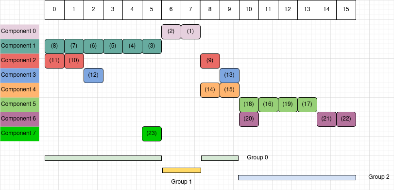
This example is illustrated Figure 1. The items are marked (1), (2),…, the order of their appearances in a walkthrough of the input data. The groups are depicted at the bottom. Please understand the problem in the diagram and compare with the result in the code above.

The code is all clean, concise, and nice. What’s surprising is that this apparently simple and uninsteresting step of processing turned out to be a dominating bottleneck of the entire program, eclipsing all the complex data pipelines and machine-learning modeling! My hunch was that the networkx algorithm was poorly crafted, whereas the problem should be relatively easy. In fact, it’s an interesting little programming problem: it’s clearly defined, rather generic, and may have a decent number of applications. Without ever looking into the networkx source code, I started developing a new algorithm for this problem.

That was a year ago, and my new algo took good parts of a day to finalize. A year later, it took me some more time to regain understanding the algo and prepare to explain it. Below is my attempt to make it understandable to you as well as to my future self.

The algorithm

Let’s assume all items across components are represented by sequential numbers from 0 up to n_items - 1, hence each component is represented by a set of such numbers. We need to work on these numbers to “union” overlapping components.

Intuiations

An ituition from the start of the effort was that it would be some kind of “sweep and mark” algorithm. There is no avoiding walking through each component with its member items, but let’s try our best to do this walkthrough only once—at least on the surface, figure out and write down relations as we go, and only do some trivial postprocessing on the findings after the single pass.

It will likely be quite procedural, with careful book-keeping along the way. Watch out for careless use of dynamic lists: create new ones, append to them, and so on. They are convenient to use, but they all take computer time! Beware of clever functional style that could triggerer recursion. I did not start thinking down that direction at all (there could be a solution in that direction but I don’t know).

So, one pass through the items. That’s the goal.

How do we represent the resultant groups? What are important intermediate relations to write down?

Eventually, each group will be represented by its member items, i.e. the sequential numbers of the items. However, as a middle step, we could also represent a group by its member components. Then it will be a cheap postprocessing to get the member items of the groups. A potential advantage is that the component-representation of groups will be small, and can lend itself to using any data structure at will, including dynamic lists, if the algo so requires.

Initial steps

Let’s stare at Figure 1. Note the items are marked by their order in the walkthrough. Suppose we walk over “component 0” first; of course it does not overlap with any previous component. Then we walk over “component 1”, again, it does not overlap with any previous component. Then we walk over “component 2” and realize it overlaps with “component 1”, hence components “2” and “1” belong to a common group.

Wait, this is easy to our eyes. But how does the code “see” the overlapping?

The code needs two “marker” lists to help with bookkeeping:

• The “item marker list” contains the “component mark” of each item. It’s a list of length n_items, denoted by C. For example, C[3] indicates the component that “item 3” belongs to. This mark starts empty (in the code we’ll use -1), and will be filled up as we walk the data.

• The “component marker list” contains the “group mark” of each component. It’s a list of length n_components, denoted by G. For example, G[2] indicates the group that “component 2” belongs to. We start with the assumption that all components are disjoint, hence the list starts as 0, 1, ..., n_components - 1.

When we walk “component 0”, we see C[7] and C[6] are empty, so we make their values 0, indicating “component 0”. Then we walk “component 1”, and assign the value 1 to C[5], C[4], C[3], C[2], C[1], C[0], noticing they have not been marked previously.

When we walk “component 2”, we first come across “item 8”, and see C[8] is not marked yet. At this moment, we would be thinking “component 0” is standing alone, “component 1” is standing alone, and “component 2” is also standing alone. Then we come across “item 1”. Boom! Its spot is already marked, as C[1] contains value 1. Immediately, we know “component 2” overlaps “component 1”. Not only “item 1”, but also “item 8”—which looked freestanding when we last visited it, as well as items of “component 2” that will come after “item 1” all belong to a group shared with “component 1”.

At this point we’ve reached the tricky part: how do we do the relationship book-keeping and all kinds of updates to it?

Think about another situation. Suppose we walk components “0”, then “1”, then “4”, and then “2”. Each of components “0”, “1”, and “4” would appear freestanding. But then “component 2” would connect the previously freestanding components “1” and “4”, triggering an update to previously-determined relations.

Wading through the tricky part

Now let’s restart the walk. At “component 0”, none of its items are previously marked, hence G[0] stays at 0. At “component 1”, similarly, G[1] stays at 1. For “component 2”, at its first item “8”, G[2] stays at 2. But at its second item “1” (step (10) in Figure 1), we see C[1] is 1, i.e, the item has been marked by “component 1”, hence the group of “component 2” should be the same as that of “component 1”, which is G[C[1]], with value 1.

Now there is a decision to be made: should we update G[1] to 2, or G[2] to 1?

To be sure, the final group numbers do not need to be consecutive numbers. They can be considered categorical labels. It turns out the group number can be either “rounded up” to 2 or “rounded down” to 1, with subsequent adjustments accordingly. We choose to round up. Hence, the list G is updated from 0, 1, 2, ... to 0, 2, 2, ....

Before moving on, I must emphasize:

The G values 0, 2, 2, ... does not mean that the group of “component 1” is “group 2”. Rather, it means that the group of “component 1” is the group of “component 2”, while the group of “component 2” is not necessarily “group 2” (although it is for now), as it may very well change later.

So we have updated the list G while visiting “item 1” of “component 2”. Then as we visit “item 0” of “component 2”, we see C[0] has value 1, and G[C[0]] has value 2. There is no update to be made here, but that’s after checking some things that are hard to understand now. Let’s move on.

Next, we walk “component 3”. First comes “item 2” (step (12) in Figure 1). We see C[2] has value 1; then checking the list G, we see G[1], or G[C[2]], has value 2, meaning “item 2” is in “component 1”, wich is in the group of “component 2”.

This is a critical moment: while walking “component 3”, we find out that it shares group with “component 1”, which shares group with “component 2”. How should we do the book-keeping?

We can update G[1] from 2 to 3. (Remember, 3 is the index of the current component.) In fact, that is optional—it’s harmless but unnecessary. What is necessary and sufficient is that we update G[2] from 2 to 3.

Why is it so?

It is possible that “component 3” does not share any item with “component 2” (and indeed that is the case). The current “item 2” could be the only opportunity that tells us “component 3” is connected with “component 2” (and indeed that is the case). If we don’t take this opportunity to record that “component 2” shares group with “component 3”, it’s possible that this info will be lost for ever. Indeed, that’s what would happen if we just update G[1] to 3 and move on, leaving G[2] with value 2.

On the other hand, it is unnecessary to update G[1] to 3. Without an update, G[1] remains 2, and continues to indicate that “component 1” shares a group with “component 2”.

The updating schme is spelt out in the pseudo-Python code below:

1
2
3
4
5
6
7
8
9
10
11
12
13
component_index = comp_i
for item_idx in item_indices_in_component_i:
    if C[item_idx] is None:
        C[item_idx] = comp_i
    else:
        comp_j = C[item_idx]
        while True:
            k = G[comp_j]
            if k == comp_j:
                G[comp_j] = comp_i
                break
            else:
                comp_j = k

In this updating scheme, the value of G[c] either remains c or gets bigger, but never gets smaller. When G[c] == c, “component c” is in “group c”. When G[c] > c, the group of “component c” is found in G[G[c]], and may need to recurse from there.

If you are somewhat lost, it may be helpful to follow Figure 2 and work through the steps.

The code

The core of the algorithm is listed below, with detailed annotations.

1
2
3
4
5
6
7
8
9
10
11
12
13
14
15
16
17
18
19
20
21
22
23
24
25
26
27
28
29
30
31
32
33
34
35
36
37
38
39
40
41
42
43
44
45
46
47
48
49
50
51
52
53
54
55
56
57
58
59
60
61
62
63
64
65
66
67
68
69
70
71
72
73
74
75
76
77
78
79
80
81
82
83
84
85
86
87
88
89
90
91
92
93
94
95
96
97
98
99
100
101
102
103
104
105
106
107
108
109
110
111
112
113
114
115
# module cc_py

from collections import defaultdict
from typing import Iterable, Sequence


def _internal(components: Iterable[Iterable[int]], n_items:int, n_components: int):
    # Each component is a sequence of items.
    # The items are represented by their indices in the entire set of items
    # across all components, hence all the elements in `components`
    # are integers from 0 up to but not including `n_items`, which
    # is the total numbe of items across all components.

    item_markers = [-1 for _ in range(n_items)]     # Component ID of each item
    component_markers = list(range(n_components))   # Group ID of each component

    for i_component, component_items in enumerate(components):
        for item in component_items:

            # Get the component ID of this item, if it has been marked
            # by a previously-visited component; otherwise it is -1.
            j_component = item_markers[item]

            if j_component < 0:
                # The item has not been marked by a previous component,
                # hence mark it by the current component.
                item_markers[item] = i_component

                # This may or may not start a new group.
                # If the `else` block below has not executed for the current
                # component, then the current component is in a new group
                # (until a later item changes this situation).
                # This new group should have the largest ID possible so far,
                # which is `i_component` (see the `else` block below).
                # The value `component_markers[i_component]` is `i_component`
                # at this moment, hence no update is needed there.
                # Since the current component is the only component in the new
                # group (for now), no update is needed to other component's
                # group IDs.
                #
                # If the `else` block below has ever executed for the current
                # component, then this component belongs to a group with ID
                # `i_component`, which has been taken care of in that block.
                # Nothing else needs to be done about the current item in addition
                # to marking it.
                #
                # Apparently, in any case, the current component belongs to group
                # with ID `i_component`.
            else:
                # The item has been marked by a previous component,
                # with ID `j_component` hence the components `i_component` and
                # `j_component` belong to the same group,
                # because they are "connected" by the current common item.
                #
                # This previous component may share its group with other previous
                # components. All these components as well as the current one
                # share a group. This block ensures that this group gets ID value
                # equal to `i_component`, and all it member components can find
                # this group ID directly or indirectly.

                # Check the group ID of the previous component.
                if component_markers[j_component] == i_component:
                    # A previous item of the current component was also marked by
                    # the component `j_component`. When the previous item was
                    # processed, it updated the group ID to `i_component` for
                    # the component `j_component`, and possibly for other connected
                    # components. All is good now.
                    continue

                # Now the current component has group ID `i_component`, but
                # the connected component `j_component` has group ID that is
                # smaller than `i_component`. Update the group ID of component
                # `j_component` and possibly others that are connected to
                # `j_component`.

                while True:
                    k_group = component_markers[j_component]
                    component_markers[j_component] = i_component
                    # This is the only line that changes `component_markers[idx]`,
                    # and the change is always upwards. Before change, the value
                    # is `idx`. After change, say `component_markers[idx] = jdx`,
                    # the component `idx` shares a group with component `jdx`.
                    # This change happens when and only when a later component
                    # (i.e. `idx < jdx`) sees that the two components are connected.

                    if k_group == j_component:
                        # This suggests the group ID for component `j_component`
                        # was never changed. Until now, the group ID for component
                        # `j_component` has been `j_component`. There may be components
                        # before `j_component` that are connected to `j_component`,
                        # but there are no components after `j_component` that
                        # are connected to it. We have updated
                        # `component_markers[j_component]` to `i_component`.
                        # We do not need to update this for components that are
                        # before `j_component` and connected to it; they will find
                        # their group ID by checking `component_markers[j_component]`.
                        break

                    # The component `j_component` is connected to another component
                    # (whose index is `k_group`) that is after it (`j_component` < `k_group`).
                    # Now that we have updated `component_markers[j_component]`, we
                    # follow the chain to update that of `k_group`.
                    j_component = k_group

    # Now `component_markers` contains the group ID of each component
    # directly or indirectly. The next block makes them all direct.
    for i in reversed(range(n_components)):
        if (k := component_markers[i]) != i:
            # Now it must be that `mark > i`, indicating
            # that the component `i` shares a group
            # with component `mark`. We follow this chain
            # to get the group ID.
            component_markers[i] = component_markers[k]

    return item_markers, component_markers

The function _internal returns the list G. It is a simple matter to finish up the algo by the following API function:

1
2
3
4
5
6
7
8
9
10
11
12
13
# module cc_py

def connected_components(components: Sequence[Sequence[int]], n_items: int):
    n_components = len(components)
    _, component_markers = _internal(components, n_items, n_components)

    groups = defaultdict(set)
    # Item IDs in each group, indexed by group ID.

    for i_comp, i_grp in enumerate(component_markers):
        groups[i_grp].update(components[i_comp])

    return list(groups.values())

Is it correct?

Let’s verify:

1
2
3
4
5
6
7
8
>>> from test import COMPONENTS_2, N_2
>>> from cc_py import connected_components
>>> COMPONENTS_2
[(7, 6), (5, 4, 3, 2, 1, 0), (8, 1, 0), (2, 9), (8, 9), (11, 13, 10, 12), (10, 14, 15), (5,)]
>>> N_2
16
>>> connected_components(COMPONENTS_2, N_2)
[{6, 7}, {0, 1, 2, 3, 4, 5, 8, 9}, {10, 11, 12, 13, 14, 15}]

Yes.

Is it fast?

For a rough benchmark, we need a way to make up some random data of somewhat realistic complexity. We used the code below to do that:

1
2
3
4
5
6
7
8
9
10
11
12
13
14
15
16
17
18
19
20
21
22
23
24
25
26
27
28
29
30
31
32
33
34
35
36
37
38
39
# module bench

import math
import time
import numpy as np
import cc_nx
import cc_py


def bench(mod, n_items, repeats=10):
    times_ref = []
    times_test = []

    for _ in range(repeats):
        n_components = int(math.sqrt(n_items))
        component_size = int(n_items / n_components * 0.8)
        components = [
                np.random.choice(n_items, component_size, replace=False)
                for _ in range(n_components)]

        t0 = time.perf_counter()
        _ = mod.connected_components(components, n_items)
        t1 = time.perf_counter()
        times_test.append(t1 - t0)

        t0 = time.perf_counter()
        _ = cc_nx.connected_components(components)
        t1 = time.perf_counter()
        times_ref.append(t1 - t0)

    print('')
    print('n_items:', n_items, 'n_repeats:', repeats)
    print('reference vs compare times (min max mean)')
    print('  ', f'{min(times_ref):.4f}', f'{max(times_ref):.4f}', f'{sum(times_ref)/repeats:.4f}')
    print('  ', f'{min(times_test):.4f}', f'{max(times_test):.4f}', f'{sum(times_test)/repeats:.4f}')


for n_items in (100, 1000, 10000, 100000, 200000):
    bench(cc_py, n_items)

Here’s the result on my old-ish Linux box, using the current networkx version 2.6.3:

1
2
3
4
5
6
7
8
9
10
11
12
13
14
15
16
17
18
19
20
21
22
23
24
n_items: 100 n_repeats: 10
reference vs compare times (min max mean)
   0.0004 0.0008 0.0004
   0.0001 0.0001 0.0001

n_items: 1000 n_repeats: 10
reference vs compare times (min max mean)
   0.0031 0.0064 0.0037
   0.0005 0.0006 0.0005

n_items: 10000 n_repeats: 10
reference vs compare times (min max mean)
   0.0334 0.0496 0.0377
   0.0049 0.0062 0.0052

n_items: 100000 n_repeats: 10
reference vs compare times (min max mean)
   0.4135 0.5574 0.4394
   0.0485 0.0702 0.0524

n_items: 500000 n_repeats: 10
reference vs compare times (min max mean)
   2.3655 2.8808 2.5499
   0.2799 0.3777 0.3075

Yes, about 8x faster than networkx. That is, of course, a great speedup by any measure.

I would like to think that my algo is near optimal. The fact that the networkx version does not really blow up as sample size increases suggests it’s not bad. It’s possible that the two algos have the same Θ complexity.

Can it be faster?

I do not see obvious ways to speed up the algorithm, but there could be ways to speed up the code. In fact, that is a consideration during the development of the algo. Pay attention to the function _internal: it’s all about navigating and updating numerical vectors of fixed sizes. Look familiar?

Yes! That’s the hallmark of computations that can be moved to C and achieve nice speedups.

We don’t have to move to C proper. Instead, we can use Numba, a Just-In-Time compiler for numerical functions in Python. Our code is revised slightly to employ Numba:

1
2
3
4
5
6
7
8
9
10
11
12
13
14
15
16
17
18
19
20
21
22
23
24
25
26
27
28
29
30
31
32
33
34
35
36
37
38
39
40
41
42
43
44
45
46
47
48
49
50
51
52
53
54
55
56
57
58
59
from typing import Sequence

import numba
import numpy as np


# Numba cache of the compiled function is in __pycache__
# in the directory of the source code.
# First run of this function includes compilation time.
# Compiling this function in particular prints a warning;
# don't worry about it.
@numba.jit(nopython=True, cache=True)
def _internal(
        item_markers: np.ndarray,
        component_markers: np.ndarray,
        i_component: int,
        component_items: np.ndarray,
        ):
    for item in component_items:
        j_component = item_markers[item]

        if j_component < 0:
            item_markers[item] = i_component
        else:
            if component_markers[j_component] == i_component:
                continue

            while True:
                k_group = component_markers[j_component]
                component_markers[j_component] = i_component
                if k_group == j_component:
                    break
                j_component = k_group


def connected_components(components: Sequence[Sequence[int]], n_items: int):
    components = [
            c if isinstance(c, np.ndarray) else np.array(c)
            for c in components
            ]
    n_components = len(components)

    item_markers = np.full(n_items, -1)
    component_markers = np.arange(n_components)

    for i, component_items in enumerate(components):
        _internal(item_markers, component_markers, i, component_items)

    for i in reversed(range(n_components - 1)):
        if (k := component_markers[i]) != i:
            component_markers[i] = component_markers[k]

    idx = (item_markers >= 0)
    item_markers[idx] = component_markers[item_markers[idx]]

    return [
            np.where(item_markers == grp)[0]
            for grp in np.unique(component_markers)
            ]

Since this version requires data to be in Numpy, we’ve also vectorized other operations in the API function. (Benchmark showed that _internal is the largest time consumer regardless of these changes.)

When benchmarking Numba code, remember to exclude the first call from timing because the first call will spend time on compilation.

Running similar benchmark code, we got the following:

1
2
3
4
5
6
7
8
9
10
11
12
13
14
15
16
17
18
19
20
21
22
23
24
n_items: 100 n_repeats: 10
reference vs compare times (min max mean)
   0.00037 0.00088 0.00046
   0.00006 0.00015 0.00008

n_items: 1000 n_repeats: 10
reference vs compare times (min max mean)
   0.00310 0.02742 0.00643
   0.00014 0.00031 0.00018

n_items: 10000 n_repeats: 10
reference vs compare times (min max mean)
   0.03354 0.06182 0.03884
   0.00043 0.00069 0.00049

n_items: 100000 n_repeats: 10
reference vs compare times (min max mean)
   0.39149 0.73823 0.45375
   0.00236 0.00354 0.00256

n_items: 500000 n_repeats: 10
reference vs compare times (min max mean)
   2.20432 2.88012 2.47352
   0.01188 0.02387 0.01466

The speedup over networkx ranges from 35 for sample size 1000 to 177 for sample size 100000. In typical situations, such speedup will turn a bottleneck to an insignificant middle step. In my case, it did just that.